In the Aquatic Fate module of CAFE, you can find fate data for chemicals in three sub-modules:

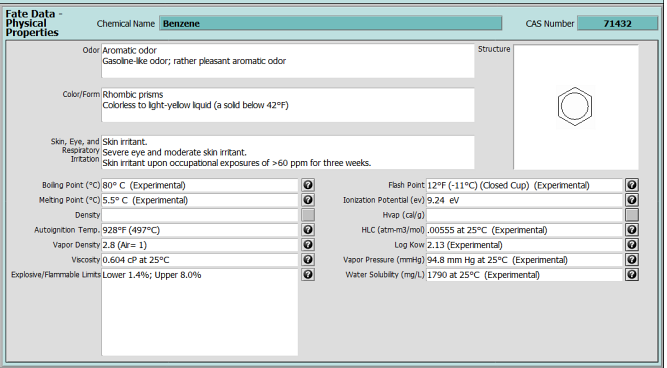
• Description and Structure: This module displays a description of the chemical and a diagram of its structure.
• Physical Properties: This module displays basic chemical information used for modeling (e.g., boiling point, water solubility, molecular weight).
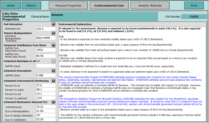
• Environmental Fate: This module displays detailed environmental explanations on the fate and behavior of individual chemicals in different media (e.g., estimated K_oc, biodegradation time, volatilization, partitioning).

NOTE: CAFE estimates both fate and effects for chemicals, but only effects for oils, dispersants, and dispersants mixed with oil.

In this example, the Structure and Physical Properties sub-module shows the chemical properties of the chemical benzene and its structure (top right). [View a larger version.]

An example from the Environmental Fate Properties sub-module for benzene. Environmental properties are shown at left, and environmental explanations on the right. [View a larger version.]

In the Aquatic Effects (Toxicity) module, you can find toxicity data for chemicals, oils, dispersants, or dispersant-oil mixtures. CAFE displays the toxicity data in the form of Species Sensitivity Distribution (SSD) curves.

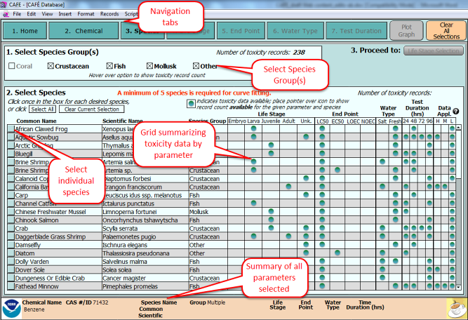
Toxicity Data Selection Work your way through the following tabs to generate a Species Sensitivity Distribution (SSD) curve:

1. Home: Select a scenario (chemical, oil only, dispersant only, or dispersant and oil).
2. Chemical: Search for the appropriate chemical, oil, dispersant, or dispersant-oil mixture and specify any additional selections.
3. Species: Select the species for which data are available (coral, crustacean, fish, mollusk, or other).
4. Life Stage: Select life stage(s) (adult, embryo, juvenile, larva, or other) for which data are available.
5. End Point: Select end point(s) (EC₅₀, LC₅₀, LOEC, or NOEC).
6. Water Type: Select water type(s) (freshwater or saltwater).
7. Test Duration: Select a test duration (24, 48, 72, or 96 hours) and applicability score(s) (high, moderate, or low), based on the relevance of these data to spill response.
8. Plot Graph: Plot your Species Sensitivity Distribution (SSD) curve.

With each step, you can see what data are available in CAFE by reviewing a toxicity grid, and then make your selections.

This example shows the Species step of an example query. You would first select Species Group(s), then select individual species. You can see what data are available in CAFE by reviewing the toxicity grid (at right). A summary of all parameters selected is displayed (bottom). [View a larger version.]

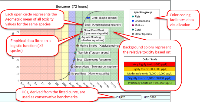
After you have completed all the steps, CAFE produces a Species Sensitivity Distribution (SSD) curve based on your selections. SSD curves are generated using the geometric mean of toxicity values (e.g., EC₅₀, LC₅₀) by species, requiring a minimum of five species per curve. SSD curves rank each species from most to least sensitive. The background colors represent the relative toxicity of each data point. Species listed towards the left of the curve (red zone) are more sensitive than species listed towards the right of the curve (green zone).

The estimated fifth hazard concentration values (HC5) are displayed for each curve and are used as conservative benchmarks under the assumption that these would be protective of 95 percent of the species on the distribution. These HC5 values are derived from each SSD curve.

This example Species Sensitivity Distribution (SSD) curve shows the toxicity of benzene to various aquatic species, based on user selections. All concentrations are plotted on a log scale and are standardized to µg/L.

The color code scheme used in CAFE's SSD curves was adopted from the U.S. EPA Office of Pesticide Programs.

Go back to the Getting Started page.